Simulated Ecology

GitHub Repo: simulatedecology

This series of programs was sparked by a challenge I found on Reddit.

The specifications are simple, and summarized briefly below:

• The World
  • Defined by user-specified width and height, or window size
  • 1 tick = 1 month
  • Simulation ends when killed by user or when deforestation is achieved
• Trees
  • Three types
    • Saplings
      • Do not produce offspring
    • Trees
      • Yield 1 lumber
    • Elder trees
      • Yield 2 lumber
  • Trees and Elder trees have a chance of reproducing every tick
    • Reproduction = place a sapling on an adjacent (diagonals included) square that is unoccupied by another tree
• Lumberjacks
  • Randomly wander around
  • Chop trees and elder trees to produce lumber
  • Every year (12 ticks) population changes
    • If surplus of wood is produced, population grows by some amount dependent on magnitude of the surplus
    • Else, fire one lumberjack to give the tree population a chance to surge again
• Bears
  • Randomly wander around
  • “Maw” lumberjacks (I suspect the correct word is “maul” and the reddit challenge misused “maw” but I am nothing if not loyal to the specifications so “maw” it is)
    • This removes the “maw’d” lumberjack from the population
  • Every year (12 ticks) population changes
    • If any lumberjacks are “maw’d” then trap one bear and send it to the zoo
    • Else, increase bear population by 1

And that’s it! Easy right?

Well… no… This is a project that I tried when it first came out. If you look at the date of the reddit post, you’ll notice that it was published in the summer of 2014. This is the summer before I began my undergraduate education at UC Irvine. As explained in the “DNA” codefolio entry, I used this summer to learn Python on my own. My first attempt at this challenge was clumsy and weak. I had not yet developed the kind of organized, sanitary coding habits that I learned while doing school projects. My code was not modular or clean and I failed to figure out an effective way to model all the behaviors listed in the specification.

But when you get knocked down, you gotta get back up.

In my 3rd year, I revisited this problem, this time with a lot more skill and experience to leverage against it. The result is Forest.py3. Here’s what it looks like:

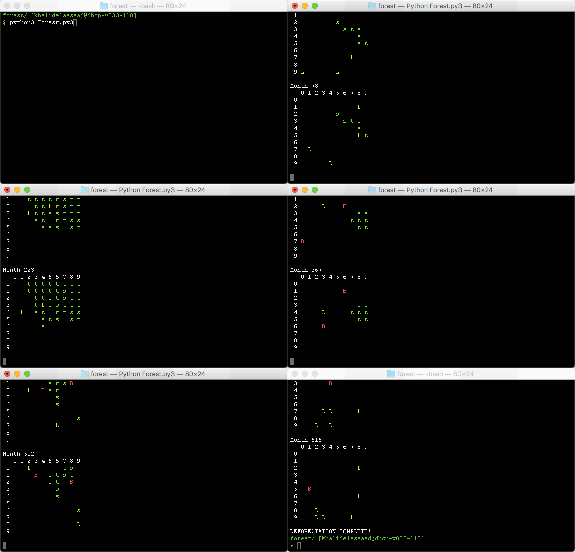
This simulation lasts 616 months. The output is printed to the terminal, which allows you to scroll up to review it.

I was very excited when this came together. The color coding gives the simulation life. I was fascinated by how the tree population would grow and dwindle, surge and ebb, teasing the edge of total deforestation a couple times before finally, in month 616, dropping entirely to 0.

However, this output system of printing everything to the terminal did not satisfy me. It especially failed to display the yearly reports that generate every 12 ticks, since the simulation would scroll past them in the blink of an eye. I wanted everything to stay in one window, so I did some research and quickly found the curses library. After some testing, I was able to throw together Forestcurses.py3. Here it is:

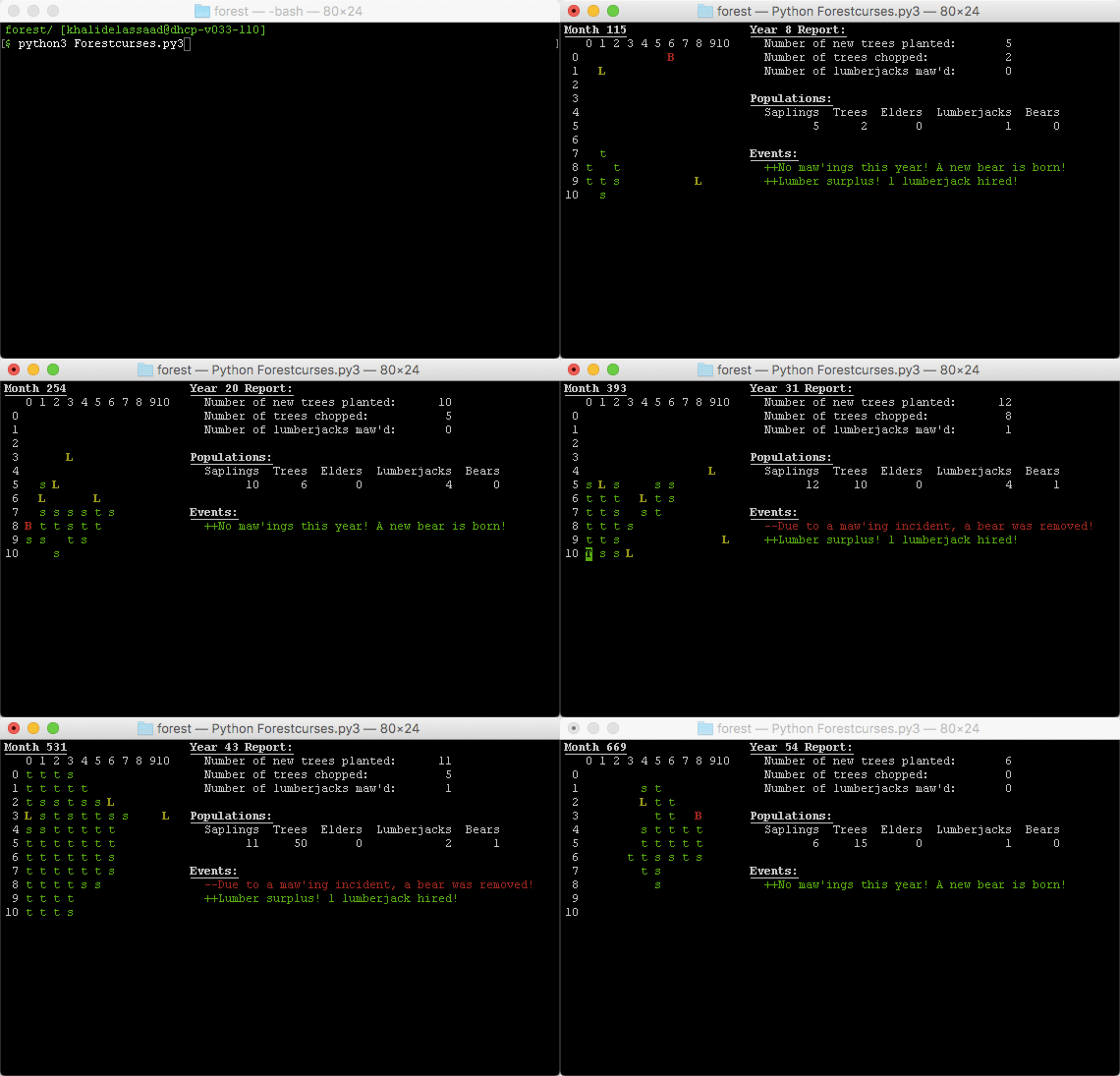
The curses library allows for a very pretty display. The yearly report is steadily visible. The user can easily keep an eye on entity populations and yearly changes to lumberjack and bear populations due to the year’s events.

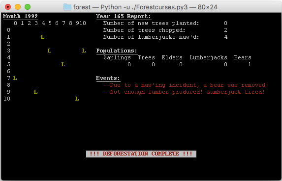
The final screen of a simulation (separate from the animated one above). A sad end to a beautiful world.

Very, very cool. A change I made in this program was to display the “T” of the elder trees as a black character on a green background. This makes them easier to spot. Elder trees are significant because they’ve survived the simulation for 10 years or 120 ticks. I also decided to keep track of “elder” lumberjacks, so we can see the 10 year survivors of that population as well. They appear as a black X on a yellow background.

The curses version of this program scales with the window size. Unfortunately so does the time it takes to compute each tick. A happy compromise between a tiny forest and a slow forest (run on an early 2014 13-inch MacBook Air) rests in the 15×15 to the 21×21 zone. For your consideration, 652 months of a 17×17 forest:

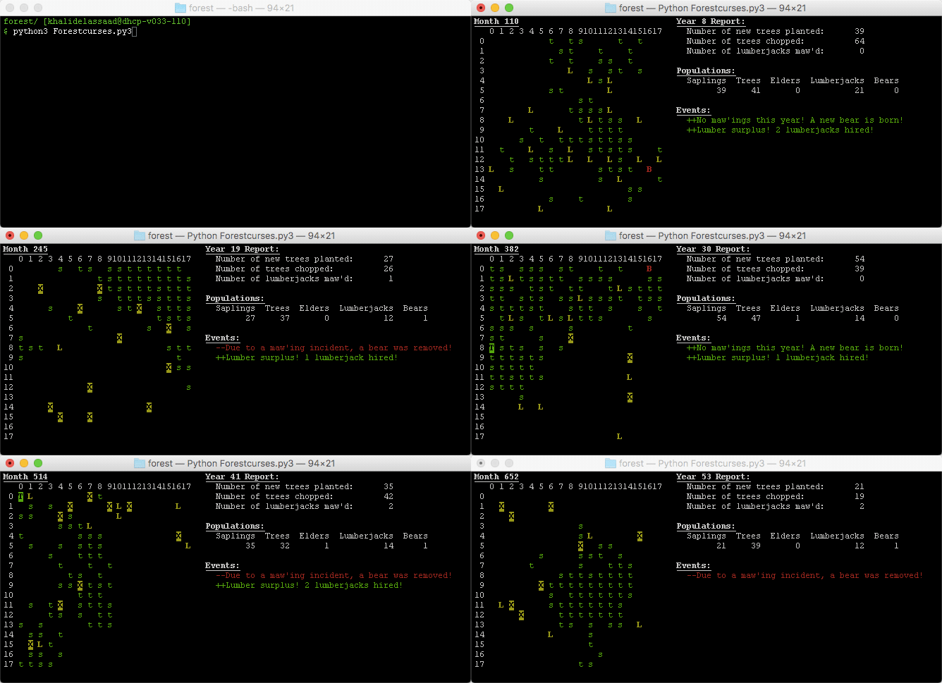
With a larger forest size, tree growth and demolition patterns are more easily observed.

Included below is a still of a 30×30 forest.

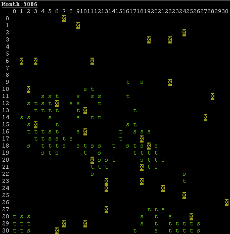
Note the organic grouping of trees. This was an immediate consequence of random generation of saplings and random wandering of tree-removing lumberjacks.

Why so many elder lumberjacks? I can come up with two reasons.

First, the simulation is in month 5006 (I left it running on accident and then walked away from my laptop for a while). There has been plenty of time for lumberjacks to age to the 120 month qualifier to become an elder lumberjack.

Second, the simulation is larger in size. The population of the trees and lumberjacks settles into equilibria that scale with the size of the simulation, such that the population density remains pretty constant regardless of simulation size (NOTE TO SELF: if I ever feel like doing a more detailed analysis, graphing population densities as a function of grid size would be pretty cool). The changes in lumberjack population are determined by the current number of lumberjacks and the amount of lumber harvested. They are dependent on a function of these values so as the values grow, the changes grow, too. The rules governing bear populations, however, are independent of the bear population. All it takes for a bear to be removed is 1 “maw’ing” incident. So even if there is only one bear in a massive 100×100 grid, if the population density of lumberjacks is at a median value, it seems from watching the simulation that it is pretty likely that the bear will collide with and “maw” at least one lumberjack in the next 12 ticks.

This results in the bear population dropping to 0! Then, for the next year (12 ticks) no “maw’ings” will occur because there are no bears, so a new bear will be born. This cycle is very likely to repeat, one year with one bear, one year with none.

Why does this result in lots of elder lumberjacks? No bears means no predators for the lumberjacks! Their survival only depends on their lumber harvest, not on luckily avoiding bears! Without a constant refresh of the lumberjack population by bears, elder lumberjacks are allowed to develop and survive!

This also means that lumberjack populations maintain a higher average value than they do at the beginning of the simulation, when the number of bears is high (because the initial number of bears is a fraction of the grid size, not just a set value). This makes deforestation a lot more likely when all the bears are removed!

Bears are good for trees, you guys! You want to save the Amazon rainforest? Breed some grizzlies and set them free!

Unrelated to any of this, I am now banned from attending environmental sustainability conferences and bear celibacy conventions.

Enough joking around, this is a serious website. And nothing is more serious than forest fires.

"Damn straight."

In late April of 2017, I was fiddling with this simulation on the road from Irvine to Sacramento to compete with my team. A teammate of mine was sitting next to me in the van, watching me code. He thought it was really cool that I could take ideas for behavior of several different units, implement them in a program, and watch the results unfold live before my eyes. I thought so, too, so I told him that we could try to take one of his ideas and implement it.

“Could you make, like, forest fires happen?”

You monster.

Great idea! The implementation of it turned out to be surprisingly simple. I added a value to a tree class member datum that indicates the “type of tree” (sapling, tree, elder, ON FIRE). Every tick, a tree on fire does one of 3 things.

1. Continues existing normally (will not be chopped down by a lumberjack)
2. Spreads its fire to an adjacent tree (1/3 probability for each adjacent tree)
3. Burns down and is removed from the simulation (1/4 probability)

Finally, every tick, every tree on the grid with at least 1 adjacent tree has a random chance to spontaneously ignite (probability 1/1000). Looking at the code now, there is a lot of looping through the lists and dictionaries that contain the grid spaces trees in order to make this happen. If I were to write this now, I would simulate the probability (1/(1000treecount)) and if the event were to occur, I would randomly select from a the tree dictionary a tree to ignite.

def firestart(self):
    fs = []
    for row in range(1,self.size):
        for col in range(1,self.size):
            if not self.notree(row,col):
                if not self.adjacenttreeless(row,col):
                    #Chance of a random fire starting
                    if not randint(0,999):
                        fs.append((row,col))
    return fs

Looping over every square and running these functions on each one is an inexcusable waste of resources. One of the problems with hobby-coding on a van is you don’t always dive into good problem solving techniques. You don’t always move past the naive solution into something smart or clever because screw it this works and it’s just a small little Python program anyways.

But enough self-whittling analysis. Let’s see it in action!

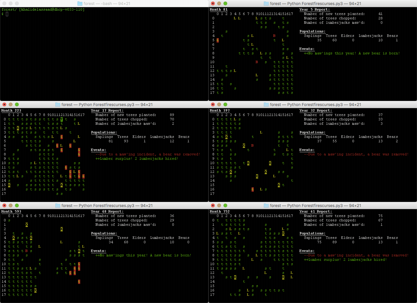
We don’t need no water let the blank blank burn. Burn blank blank. Burn.

How cool is that? In some parts of the simulation (like around month 585), there are two distinct colonies of trees that seem like they will grow into each other and connect. Suddenly, a fire will start and demolish one completely, leaving the other unaffected.

I’m left saddened that the two colonies never connected but relieved that at least one survived, an unlikely outcome had the gap between them been bridged. Truly humbling.

Sometimes, the opposite happens. It is more likely in larger simulations. A large colony of trees will ignite on one end and the fire will begin to spread. Sometimes, almost as if in response, a wave of lumberjacks will chop through the center of the colony, splitting it into two. The burning half is annihilated in the blaze, but the other half survives and grows again. This wasn’t planned when I wrote the code, and it wasn’t even the intended behavior of the lumberjacks (since they move randomly), but sometimes you get unpredicted behavior when you code.

Simulations like these can sometimes be a lot of work. You put thought and effort into modeling the behaviors of different objects, all of which will be tiny units in the simulation. When the time comes to put a bunch of them together in a box and let them play with each other, you never really know what’s going to happen. The uncertainty is exciting and the pay-off of watching your code do something that you had not anticipated is surprisingly thrilling.